CSE202 HW3
Problem 1
Idea
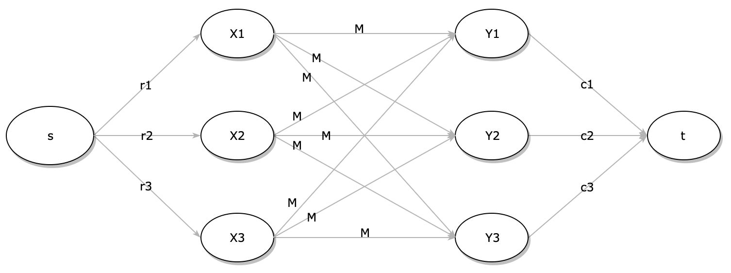
We can think every row as a node with influx of row’s sum that we want to distribute into every column which is also a node with edge’s capacity of M.
Let’s define $X_1 … X_n$ to be the rows and $Y_1 .. Y_n$ to be the columns. The preliminary graph looks like this.
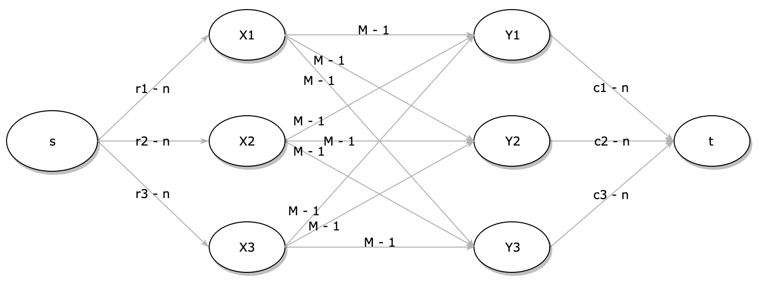
Due to the nature of the network flow problem, we might have edge with 0 flow. However, in our problem we have constraint of filling number between 1 to M. Therefore, we need to reduce the edge connecting X to Y with reduced capacity of M - 1, and add 1 back later. Because we reduce the edge’s capacity, we also need to reduce influx of every X by number of columns, which is equivalent of deducting 1 for every cell. Meanwhile the efflux of the Y will need to be reduced by the by number of rows. With these considerations in mind, we update the graph to below.
Algorithm
ALGO(M, $r_1…r_n$, $c_1…c_n$):
- G(V, E) = contructGraph(M, $r_1…r_n$, $c_1…c_n$)
- f = MaxFlow(G(V,E))
- a = array of n x n
- fill a according to: $a_{ij} = 1 + f(X_i, Y_j)$
- if $\sum_i a_{ij} = c_j$ for $1 \leq j \leq n$ and $\sum_j a_{ij} = r_i$ for $1 \leq i \leq n$
- return a
- else
- return “Impossible”
Analysis
Time Complexity
The best time complexity for MaxFlow take $O(n^3)$ using Pre-Flow Push Algorithm, where n = number of vertices. The time for filling the entry and check takes $O(n^2)$. So overall time complexity is $O(n^3)$.
Space Complexity
No extra space besides a is use, so space complexity O(1).
Correctness
Since the preliminary graph contains correct influx for all the rows and correct efflux of the columns. We essentially making sure all the sums are capped with the corresponding sum. With edge capped with M, we make sure no edge can have value greater than it. With consideration of potential 0 flow, we come up with modified graph where deduct the $X_i - Y_j$’s capacity by 1. We also adjust all the influx and efflux according to make sure the conservation of influx and efflux.
After the program completes, we simply add the 1 back to flow to accommodate the modification made above. So all the constraints in the problem are strictly enforced to guarantee the correctness of the algorithm.
Problem 2 (KT 6.11)
Idea
Let OPT[i] denote the minimum cost for cost up to week i. For each week i, we have choice of either using A or B. So the OPT[i] reduces to following:
$$ OPT[i] = \begin{cases} OPT[i - 1] + r * s_i \newline OPT[i - 4] + 4 * c \newline \end{cases} $$
which is then reduces to following
$$OPT[i] = \min(OPT[i - 1] + r * s_i , OPT[i - 4] + 4 * c)$$
Algorithm
ALGO(n, s, c):
Let OPT = array of 0’s with size n + 1
Let OPT[i] = 0 $\forall i \leq 0$
for i = 1 to n
- OPT[i] = min(OPT[i - 1] + r * $s_i$ , OPT[i - 4] + 4 * c)
return OPT[n]
Analysis
Space Complexity
OPT takes O(n).
Time Complexity
We only have 1 loop which iterates up to n, so O(n).
Correctness
Base case when i = 0, OPT[i=0] = 0. Now for any other i > 0, assume the OPT[i - 1] and OPT[i - 4] contains the correct minimum cost for week i - 1 and i - 4 respectively by induction. Now for week i, we can either continue use company A with cost of OPT[i - 1] + r$s_i$ or we can rethink our strategy and use company B instead with OPT[i - 4] + 4c cost.
Problem 3 (KT 7.5)
False. The (A,B) is no longer the minimum cut. Consider the following example.
Initially $A^*$ = {s, a, b, c, d} with c(A,B) = 3, if we increase the weight by 1 to every edge the new $A^*$ = {s} with c(A,B) = 5.
Problem 4
Idea
The find the maximum grade, we can spend 0 up to H hours for each project, then if we do decide to spend h hour for the first project, then we have H - h hours for other project. This leads to a natural recursion algorithm.
Or we can use dynamic programing to save the intermediate result, where we create an dp array of k by H. Each dp[i, j] represents the maximum grade for spending j hours for project from 1 to i.
Algorithm
ALGORecursive(H, G):
- if length of G = 1, return $G_1[H]$
- BestGrade = 0
- for h = 0 to H
- Grade $\gets G_1[h] + ALGO(H - h, G[2:k])$
- BestGrade = max(Grade, BestGrade)
- return BestGrade
ALGOIterative(H, G):
- DP=array of k by H
- for h = 0 to H
- DP[1, h] = $G_1[h]$
- for p = 2 to k
- for $h_1$ = 0 to H
- BestGrade = 0
- for $h_2$ = 0 to $h_1$
- Grade = $G_p[h_2] + DP[p - 1, h_1 - h_2]$
- BestGrade = max(BestGrade, Grade)
- $DP[p, h_1]$ = BestGrade
- for $h_1$ = 0 to H
- return DP[k, H]
Analysis
Time Complexity
There are three nested loops with length of k, H, H, so runtime = $O(kH^2)$.
Space Complexity
Depends on the algorithm use, if we use recursion we have O(1) otherwise we have O(kH). Moreover, we can even further reduce the dp method to use only O(H) since we only rely on the row.
Correctness
Base case, when we have only k = 1 project, we need to spend all H hours to the project to get the maximum grade, since $G_i[H] \geq G_i[H- 1] \geq … \geq G_i[0]$. For any i > 1, assuming we have all the correct result for i - 1 projects by induction. For this project, we can spend from 0 up to H hours on project i. Now if we spend h hour on project i, we only have H - h hours left, then we just have to check which h and H - h combo resulting the best grade and this is the answer ties to 1 to i projects with total hour H.